Scale-aware Auto-context-guided Fetal US Segmentation with Structured Random Forests
1National-Regional Key Technology Engineering Laboratory for Medical Ultrasound, Guangdong Key Laboratory for Biomedical Measurements and Ultrasound Imaging, School of Biomedical Engineering, Health Science Center, Shenzhen University, Shenzhen 518060, China
2Department of Electronic Engineering, the Chinese University of Hong Kong, Hong Kong, China
*Correspondence to: Dong Ni and Li Liu, E-mail: nidong@szu.edu.cn; liliu@cuhk.edu.hk
Received: May 20 2020; Revised: August 18 2020; Accepted: September 9 2020; Published Online: September 29 2020
Cite this paper:
Xin Yang, Haoming Li, Li Liu and Dong Ni. Scale-aware Auto-context-guided Fetal US Segmentation with Structured Random Forests. BIO Integration 2020; 1(3): 118–129.
DOI: 10.15212/bioi-2020-0016. Available at: https://bio-integration.org/
Download citation 
© 2020 The Authors. This is an open access article distributed under the terms of the Creative Commons Attribution License (https://creativecommons.org/licenses/by/4.0/). See https://bio-integration.org/copyright-and-permissions/
Abstract
Accurate measurement of fetal biometrics in ultrasound at different trimesters is essential in assisting clinicians to conduct pregnancy diagnosis. However, the accuracy of manual segmentation for measurement is highly user-dependent. Here, we design a general framework for automatically segmenting fetal anatomical structures in two-dimensional (2D) ultrasound (US) images and thus make objective biometric measurements available. We first introduce structured random forests (SRFs) as the core discriminative predictor to recognize the region of fetal anatomical structures with a primary classification map. The patch-wise joint labeling presented by SRFs has inherent advantages in identifying an ambiguous/fuzzy boundary and reconstructing incomplete anatomical boundary in US. Then, to get a more accurate and smooth classification map, a scale-aware auto-context model is injected to enhance the contour details of the classification map from various visual levels. Final segmentation can be obtained from the converged classification map with thresholding. Our framework is validated on two important biometric measurements, which are fetal head circumference (HC) and abdominal circumference (AC). The final results illustrate that our proposed method outperforms state-of-the-art methods in terms of segmentation accuracy.
Keywords
Automatic measurement, contour enhancement, fetal biometrics, structured random forests, ultrasound image segmentation.
Introduction
Ultrasound (US) imaging has been widely employed in prenatal diagnosis due to its superior advantages, such as real-time imaging, low-cost and mobility. To evaluate the fetal development and gestational age (GA), fetal biometry measurements are needed during US examinations, such as fetal head circumference (HC) and abdominal circumference (AC).
Manually delineating the fetal anatomy boundary to get those biometrics is necessary for fetal biometric interpretation from US images.
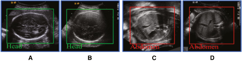
In reality, it is difficult for the clinician to delineate the edge manually, which is time-consuming and often results in large inter- and intra-observer variability [1]. Thus, an automatic approach for boundary segmentation is highly demanded for improving clinical work-flow and diagnosis objectiveness. However, there are several challenges for the segmentation algorithm of fetal anatomy from US images. First of all, the US image quality is often affected by various intensity distributions due to different imaging conditions. Secondly, several factors including acoustic shadows, speckle noise and low contrast between objects and surrounding tissues cause the typical boundary ambiguities and long-span occlusion [2], as shown in Figure 1. Last but not least, deformation of fetal anatomical structures might occur as a result of different pressure sources.
Figure 1 Standard planes of the fetal head (A, B) and abdomen (C, D) in ultrasound. The fetal head has a clearer boundary than the fetal abdomen, but suffers greater inner structural changes than the fetal abdomen as gestational age increases.
For the aforementioned issues, a number of researches for automatic fetal anatomy segmentation in US have been conducted.
Extensive attempts in recent works can be mainly classified into the following four categories.
- Semi-automatic segmentation methods. Yu et al. [3, 4] proposed a semi-automatic solution by using a gradient vector field-guided snake to obtain the real edges of the fetal abdominal contour in US images. Ciurte et al. [5] proposed formulating the task of fetal head segmentation as a continuous minimum cut problem. However, semi-automatic solutions require a user-assisted labeling process to initialize the segmentation, hence making the measurement process tedious and subjective.
- Shape model-based methods. Jardim et al. [6] proposed a region-based maximum likelihood formulation of parametric deformable contours for fetal femur and head measurement in US images. Wang et al. [7] applied an iterative randomized Hough transformation to fit the fetal abdominal contour in US images. Wang et al. [8] combined an entropy-based segmentation method with a shape-prior model to segment fetal femur from US images. Foi et al. [9] designed an elegant fetal head model (DoGEll) and formulated the fetal head segmentation as an ellipse model fitting problem. Specifically, this method minimized a cost function by a multi-start multi-scale Nelder-Mead algorithm to segment the fetal head from US images. The cost function was based on the assumption that the intensities of the pixels of the skull are on an average greater than the surrounding tissues. However, this hypothesis may not always be correct owing to the appearance of surrounding tissues with high intensities.
- Learning-based methods.
- – Regression-based methods. One closely related research is the regression-based method, which has a similar goal of automatic anatomical segmentation and landmark detection. For example, Gall et al. [10] used a Hough forest to directly map the image patch appearance to the possible location of the object centroid. More recently, Namburete et al. [11] used regression forests to build the mapping between US image appearance and GA. In their study, Gao et al. [12] introduced the regression forests for context-aware multiple landmark detection in prostate computed tomography (CT) images. In order to segment prostate in CT images, Gao et al. [13] also proposed to use the popular regression forests to learn the transformation between patches’ appearance and their three-dimensional (3D) displacement to the nearest boundary points. However, as general feature representation methods tend to lose their power in distinguishing patches of fetal US, simple distance information labels are ineffective in driving the complicated regression process.
- – Classification-based methods. Yaqub et al. [14] used weighted random forests for classification and segmentation in fetal femoral US image. However, this traditional pixel-wise classification scheme will lead to information loss in those boundary-missing areas. This is why structured random forests (SRFs) are introduced for US image segmentation based on patch-wise prediction, inspired by [15, 16]. SRFs can directly map a patch to its segmentation, that is, it can predict the labels of all pixels within a patch simultaneously, including those pixels in boundary-missing areas. Domingos et al. [17] proposed to use SRFs to transfer an US patch into its segmentation directly. A structured label greatly boosts this kind of transfer, but how to choose the optimal patch scale and maximize the ability of fitting all contour details remains to be a challenge.
- Integration of shape model-based and learning-based methods. Model-based and learning-based methods have their own limitations. Model-based methods usually provide acceptable results. However, their training processes require a large number of data. In contrast, learning-based methods perform well when only a small dataset is available. However, they largely rely on precise initialization and are also susceptible to errors. Some recent works tend to integrate both methods to achieve better performance. For example, Carneiro et al. [18] employed a constrained probabilistic boosting tree for automatically detecting fetal anatomies, which directly exploits a large dataset of fetal anatomical structures in US images with expert annotation. However, there are still 20% of the automatic measurements in [18] showing relatively large errors because of a great divergence in appearance between the testing and training images. Recently, Ni et al. [19] used ellipse fitting to measure the fetal HC based on learning-based methods.
In this paper, we mainly focus on two aspects to compose an automatic solution for accurate segmentation of fetal anatomical structures in US images, with the following contributions:
- The SRF is used as the core discriminative classifier to transfer the intensity image into a classification map and recognize the region of fetal anatomical structure. Specifically, the patch-wise joint prediction presented by the SRF is excellent in differentiating an ambiguous boundary and reconstructing a missing boundary, which is highlighted as a great advantage over traditional pixel-wise classifiers.
- In order to get a more accurate classification map, a scale-aware auto-context model (SACM) is injected to enhance the contour details of the classification map from various visual levels. Different from the classical auto-context model (ACM), each level in our model will focus on rendering the map with a level-specific scale, which is aimed at mining more map details successively. Additionally, the modified map from the previous level will not only provide important contextual information but also a strong spatial constraint for the following levels, and thus make classifiers be more specific to classify boundary patches. After the iterative refinement, the final classification map will become converged and smooth enough, and thresholding will be applied to obtain the final segmentation.
The remainder of this paper is conducted as follows. We first describe the details of our framework in the “Methods” section, and then present the experimental results of the proposed method in the “Experiment” section. Finally, the “Experimental Results and Discussion” section elaborates the discussion and conclusions.
Methods
System overview
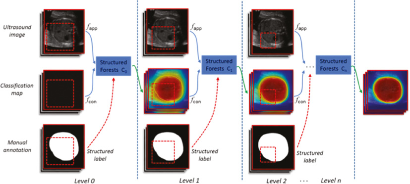
Our proposed method is composed of two critical components, that is, the SRFs and the SACM. Specifically, the SRFs are first used as the core discriminative classifier to effectively predict the fetal head or abdominal regions, where the initial probability maps are obtained. Then, to get a more smooth classification map, a SACM is injected to enhance the contour details of the classification map from various visual levels. The final segmentation can be obtained from the converged classification map with thresholding. Figure 2 gives an illustration of our framework.
Figure 2 Full illustration of our framework. From the level-specific scale patches, shown as red dotted box, the appearance feature (fapp) and context feature (fcon) are extracted. In the training stage, extra structured labels are collected from manual annotations. In the testing stage, all classifiers will be sequentially applied on the testing image for prediction and refinement.
Randomized Haar-like feature extraction
Haar-like features have been widely used in US image processing [20–22] due to their robust representation of noisy US images. Generally, conventional Haar-like features [23] are extracted from the training samples to represent the appearance of the anatomical structures. However, in this study, we use the random Haar-like features (RHaar) [13] not only for appearance features but also for context features. Considering the efficiency, our implementation employed the integral image technique [23] to speed up the calculation of the RHaar features. Specifically, for each pixel (m, n), its RHaar features are denoted as follows:
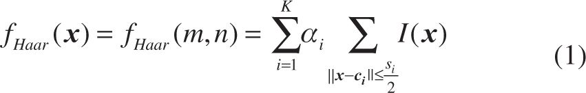
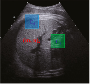
where K denotes the number of the used rectangles; αi ∈ {+1, −1} denotes the combination coefficient; ci and si denote the center coordinate and the size of the rectangle, respectively; I(x) is the intensity of the pixel x. Therefore, we can generate multiple features by randomly choosing K, αi. ci and si. In this paper, we set K = 2. As shown in Figure 3, the RHaar features at the pixel (m, n) include not only local appearance information, but also contextual information due to any two randomly displaced rectangle regions (see C0 and C1).
Figure 3 Randomized Haar-like features.
SRF boosted classifier
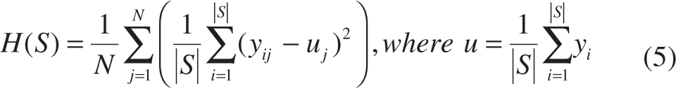
Random forest
As a classical learning-based method to address classification and regression issue, random forest has been widely adopted in medical imaging applications [24]. Random forest comprises multiple decision trees. At each internal node of a tree, a feature is chosen to split the incoming training samples to maximize the information gain. Specifically, let x ∈ X ⊂ Rq be an input feature vector, and c ∈ C = {1, …, k} be its corresponding class label for classification based on feature representation f(x). The random forest is an ensemble of decision trees, indexed by t ∈ [1, T], where T is the total number of trees at each iteration. A decision tree consists of two types of nodes, namely internal nodes (non-leaf nodes) and leaf nodes. Each internal node stores a split (or decision) function, according to which the incoming data is sent to its left or right child node, and each leaf stores the final answer (predictor). More specifically, for a given internal node i and a set of samples Si ⊂ X × Y, the information gain achieved by choosing the features to split the samples in the N-class classification problem (N ≥ 1) is computed by:
H(S) denotes the Shannon entropy, and pn is the frequency of the class n in S.
During the training process, the splitting strategy is implemented recursively until the information gain is not significant, or the number of training samples falling into one node is less than a pre-defined threshold.
Structured random forest
Recently, SRFs [7] have emerged as an inspiring extension of random forests [8].
Instead of stepping through mask patches to extract abstract or high semantic-level cues to serve as learning targets, SRFs take whole mask patches as targets directly, referred to as a structured label (Figure 4). The informative structured labels magnify the dissimilarity between patches in the target space and significantly remove the ambiguity in labeling. The distinctive structured labels strongly boost the training of weak learners in split nodes (Figure 4). Consequently, with the learned straightforward mapping from intensity patches to their segmentations, SRFs can present attractive patch-wise prediction, that is, all pixels within an unseen patch can be labeled jointly. The patch-wise joint prediction is important for boundary prediction in fetal US, because those pixels located around ambiguous or missing boundaries can only be co-labeled with the support from neighbors.
For the training of SRFs, we denote S = X × Y as the training data for a tree in SRFs, X and Y are the feature matrix and target matrix, respectively. St ⊂ X × Y is the training data of the split node t. The best weak learner in the split node t is acquired by optimizing the general objective function:
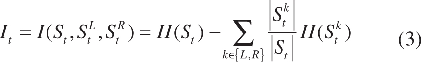
where  , and H(S) is used to measure the consistency of targets in S.
Traditionally, for the N-class classification problem (N ≥ 1):
H(S) denotes the Shannon entropy, and pn is the frequency of the class n in S.
For the N-dimensional regression problem (N ≥ 1):
SRFs will be considered as an N-dimensional regression problem if we take structured labels as simple long vectors. However, it is quite computationally expensive to calculate H(S) as in Equation (5) in each split node for high-dimensional structured labels, and it is not accurate to measure the consistency with Equation (5) for SRFs, because there exist high correlations between elements in structured labels, while H(S) in Equation (5) ignores those with averaging.
Figure 4 Toy example illustrating the weak learner training procedure of SRFs. Patches are accompanied with their structured labels. In SRFs, driven by structured labels, those patches can be clustered into two distinct subsets easily by the weak learner.
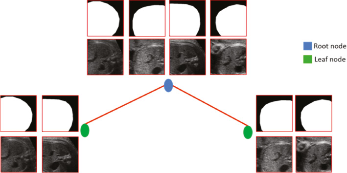
Considering the computational cost and difficulties in defining accurate consistency metrics for structured labels, in this paper, we propose to re-label each intensity patch by transferring their structured labels into a discrete set of labels c ∈ C, where C = {1, …., k}. Specifically, this re-labeling only occurs independently in each split node, and structured labels can preserve their dissimilarities to guide all splitting procedures. Finally, training SRFs can be converted into a classical N-class classification problem and share the same definition of H(S) in Equation (4). In our method, the K-means algorithm is adopted for the direct re-labeling, and we set the cluster number k to 2 [see Figure 5(A)].
Figure 5 (A) Dimension reduction using K-means algorithm in split nodes. (B) Fusion result of all patches using the fusion strategy where the probability of each pixel is the average of all pixels from overlapping patches.
Ensemble model
With the representative RHaar features and informative structured labels, the SRF model can be trained efficiently. In the prediction stage, once an unseen patch reaches a leaf node after a series of binary tests with weak learners, all structured labels stored in the leaf node will be averaged to form a classification map. The final classification result for a patch is the average of all classification maps across all tress in the SRFs. The final classification result for the whole image is the fusion result of all patches using the fusion strategy as illustrated in Figure 5(B), where the probability of each pixel is the average of all pixels from overlapping patches.
Scale-aware auto-context model-guided detail enhancement
Although our the SRF classifier can output more reasonable classification probability map than traditional pixel-wise prediction methods, the details in the map still need to be improved, as the level 1 classification map in Figure 2.
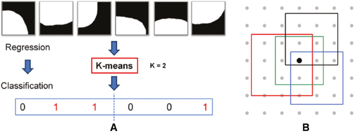
The classical ACM [19] is famous for its generality in exploring both the appearance and contextual feature to refine the details of the primary prediction result, and among the two kinds of features, the contextual feature contributes most to the final incremental refinement. However, the classical ACM uses a fixed scale through all model levels to compute the appearance feature and the context feature, which is considered to be improper in our fetal US applications. Because of suffering from the ambiguous and missing boundary in US, we need to get a global appearance feature from large-scale patches to give a basic location guidance of fetal anatomy. We also need the appearance feature from small-scale patches to fit local details. Most importantly, the contextual feature that we refer to should be different when we focus on the classification in different scales. Computing the contextual feature with a large scale is good at capturing holistic geometric distribution existing in the classification probability map of the previous level, while the contextual feature from a small scale is more appropriate in describing local distribution. Choosing an optimal patch scale in extracting those two kinds of feature is a tough task, especially in low-resolution US images. Additionally, error accumulation is another limitation for traditional ACM. Specifically, if significant prediction errors occur in the early level, errors will increase gradually and not be corrected effectively in subsequent levels due to the fact that subsequent iterations severely depend on contextual information of the previous level. Figure 6 shows the prediction results in traditional ACM using the image patches (30 × 30) to extract the appearance feature and the context feature for training a multi-level classifier. We can observe that subsequent iterations cannot correct error if the prediction of the first level has obvious misclassification (white arrow).
Figure 6 Error accumulation in ACM where the yellow contour represents the ground truth of the fetal abdomen.
To address the aforementioned problems and get more accurate classification results, we propose to integrate the SRFs with a SACM.
In the training stage, compared to the classical ACM, our model extracts the appearance feature and the context feature with a level-specific patch scale to learn from different visual levels. Specifically, the patch scale decreases gradually with the increase in the model level (see Figure 2). In the early levels, SRFs will learn to explore global appearance information and contextual information to figure out the basic shape of fetal anatomy with a coarse classification map. With an increase in the model level, SRFs will gain more ability in fitting map details by introducing local appearance and contextual information. Additionally, to make the training focus more on the boundary patches, SRFs in level i(i ≥ 1) will only learn from the patches around boundaries with the boundary cues obtained from the classification probability map of level i−1. In this paper, we use morphological operators on the classification map of level i−1 to produce an edge band as the cues, as shown in Figure 7. Similar to the appearance feature, RHaar-like filters are adopted to encode context information.
Figure 7 Illustration of SACM where the classification probability map of the previous level is used to extract patches around the boundary of the fetal ROI.
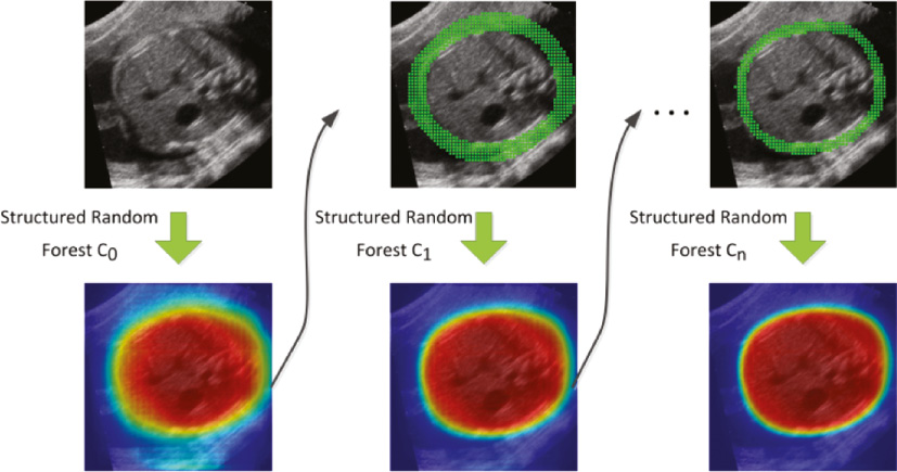
In the testing stage, all SRFs classifiers trained with our model will be sequentially applied to the testing image and will initially pick out the fetal anatomy from a complex background with a roughly estimated map. Then, the details of the classification map, especially boundary details, will be iteratively enhanced from different visual levels until convergence. Thresholding will be applied on the converged classification map to obtain the final segmentation result.
Fetal biometric measurement
Based on the segmentation results described in the previous sections, we can estimate biometric measurements, which are the values used clinically for fetal growth assessment. In this paper, we estimate the fetal HC and AC measurement derived from the segmentation objects, reported in millimeters, using the resolution information of each US image.
Experiments
Datasets
We validate our framework on two tasks with two datasets. Both of them are important for pregnancy evaluation and exhibit different challenges to computer-aided segmentation algorithms [25], as described in the following:
- The fetal head dataset is our in-house data. In the training stage, a total of 300 cropped fetal head standard plane images (128 × 128 pixels) [21] associated with complete manual annotations are provided for training, where 40 patches are sampled from each image. In the testing stage, a total of 236 fetal head standard plane images (768 × 576 pixels) are provided for head segmentation. For both training and testing, the fetal head dataset has a GA from 20 to 36 weeks.
- The abdomen dataset is our in-house data as well. In the training stage, a total of 398 cropped fetal abdomen standard plane images (128 × 128 pixels) associated with complete manual annotations are provided for training, where 40 patches are sampled from each image. In the testing stage, a total of 505 fetal abdomen US images (768 × 576 pixels) are provided for abdomen segmentation. For both training and testing, the fetal abdomen dataset has a GA from 18 to 40 weeks.
For both datasets, due to the fact that the fetal head and abdomen are moving objects in the uterus [10], we first use the random forests classifiers to localize the coarse region of interest (ROI) of the fetal head and abdomen from standard planes automatically and then resample the ROI images to the same size with training images for segmentation. For objective evaluation, all testing images have ground truth provided by two experienced doctors.
The following parameter settings were used for all experiments throughout this paper, if not mentioned specifically:
- Number of levels in our SACM: 4
- Patch size in Level 0: 90 × 90 pixels
- Patch size in Level 1: 76 × 76 pixels
- Patch size in Level 2: 50 × 50 pixels
- Patch size in Level 3: 30 × 30 pixels
- Cluster number k used in the SRF: 2
- Number of trees in each level: 10; maximum tree depth: 25
- Threshold used in the SRF: 0.7
Quantitative measurements
To comprehensively evaluate the segmentation accuracy, we used two types of metrics:
- Region-based metrics (precision, recall and dice)
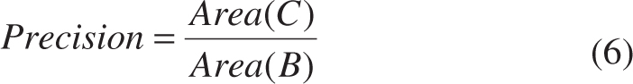
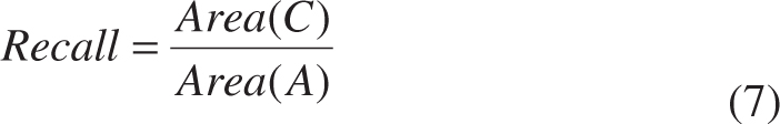
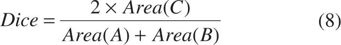
where Area(*) is an operator for area computation, A is the ground truth provided by experienced experts, B is the segmentation results obtained from algorithms, and C is the overlap between A and B [see Figure 8(A)].
- Distance-based metrics [maximum surface distance (MSD), average surface distance (ASD) and root mean square surface distance (RMSD)].

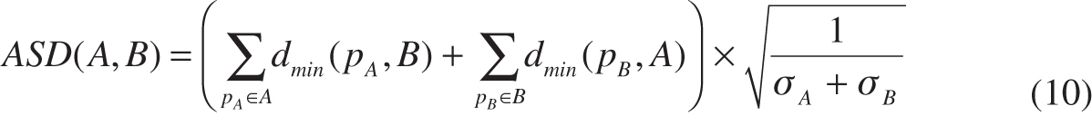
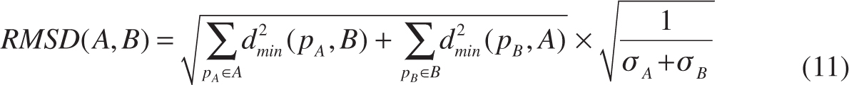
where A is the ground truth for image contour on which the number of points is σA, B is the image contour computed by an algorithm on which the number of points is σB. dmin(pA, B) denotes the shortest distance between the point pA on the contour A and the point on the contour B. Similarly, dmin(pB, A) denotes the shortest distance between the point pB on the contour A and the point on the contour B [see Figure 8(B)].
Figure 8 (A) Region-based evaluation metrics; (B) distance-based evaluation metrics.
Statistical analysis
The Kolmogorov-Smirnov test was used as the data normality strategy. Linear regression was commonly used to acquire the correlation between the segmentation outputs obtained by our method and the annotation. For linear regression analysis, the independent variable was defined as the segmentation results (fetal HC and AC) obtained by our method. The dependent variable was defined as the ground truth obtained by experienced doctors. The strength of the correlation was assessed using the Pearson correlation coefficient, r, which was interpreted as follows: very weak if r = 0–0.19, weak if 0.20–0.39, moderate if 0.40–0.59, strong if 0.60–0.79 and very strong if 0.80–1.00 [26].
Experimental results and discussion
Qualitative assessment
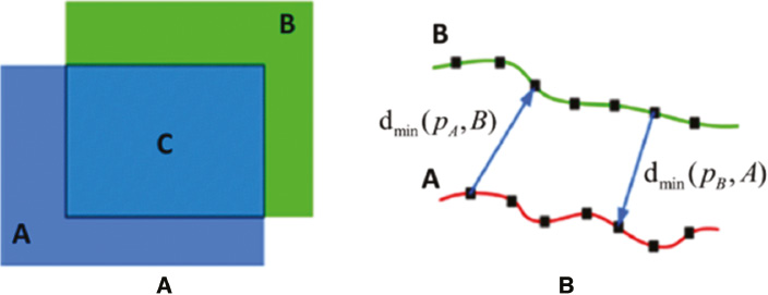
As shown in Figure 9 and Figure 10, qualitative evaluation of the segmentation results computed by our method was conducted. We can see that the classification maps in early context levels are excellent in capturing the coarse shapes of the fetal head and abdomen, and the residuals between our segmentation results and ground truth are reduced gradually as the context level increases.
Figure 9 Classification probability map with context levels 0, 1, 2 and 3 (from left to right).
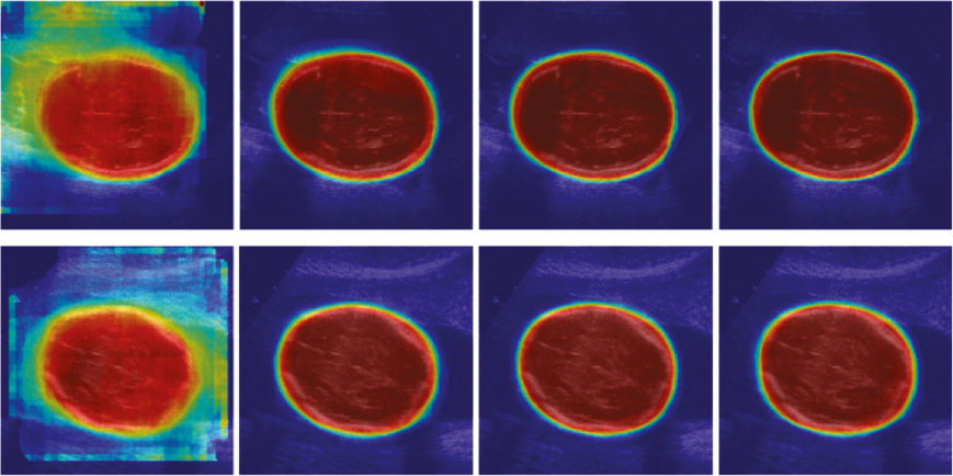
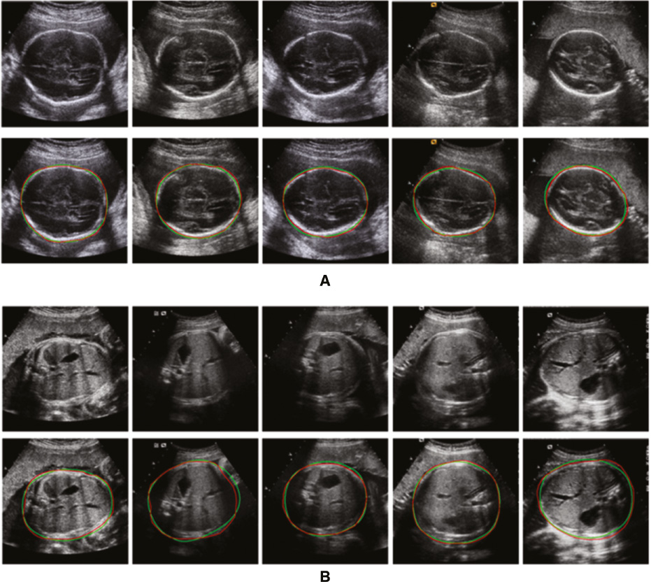
Figure 10 Qualitative segmentation results of (A) the fetal head and (B) the abdomen ultrasound images. The red line denotes the ground truth; the green line denotes the results of our method.
Quantitative assessment
Comparison of the segmented fetal HC and AC between our method and manual delineations by two doctors showed similar results. Regression analysis quantitatively showed that the segmentation outputs obtained by our method had good correlation with those obtained by manual delineations from two experienced doctors, which were taken as the ground truth. Specifically, a very strong correlation was found between the segmented HC obtained by our method and the ground truth (r = 0.97 > 0.8, p < 0.001) [Figure 11(A), (C)], while a very strong correlation was also found between the segmented AC obtained by our method and the ground truth (r = 0.92 > 0.8, p < 0.001) [Figure 12(A), (C)].
Figure 11 Scatter plots of the fetal head circumference (HCs) obtained automatically by our proposed method against those obtained manually by the first (A) and the second (C) experienced doctors; Bland-Altman plots for fetal HC. Each graph visualizes the difference between the automatically and the manually obtained HC by the first (B) and the second (D) experienced doctors. The difference in HC is distributed evenly around the zero line and within clinically acceptable 95% confidence intervals.
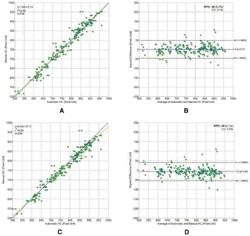
Figure 12 Scatter plots of the fetal abdomen circumference (ACs) obtained automatically by our proposed method against those obtained manually by the first (A) and the second (C) experienced doctors; Bland-Altman plots for fetal AC. Each graph visualizes the difference between the automatically and the manually obtained AC by the first (B) and the second (D) experienced doctors. The difference in HC is distributed evenly around the zero line and within clinically acceptable 95% confidence intervals.
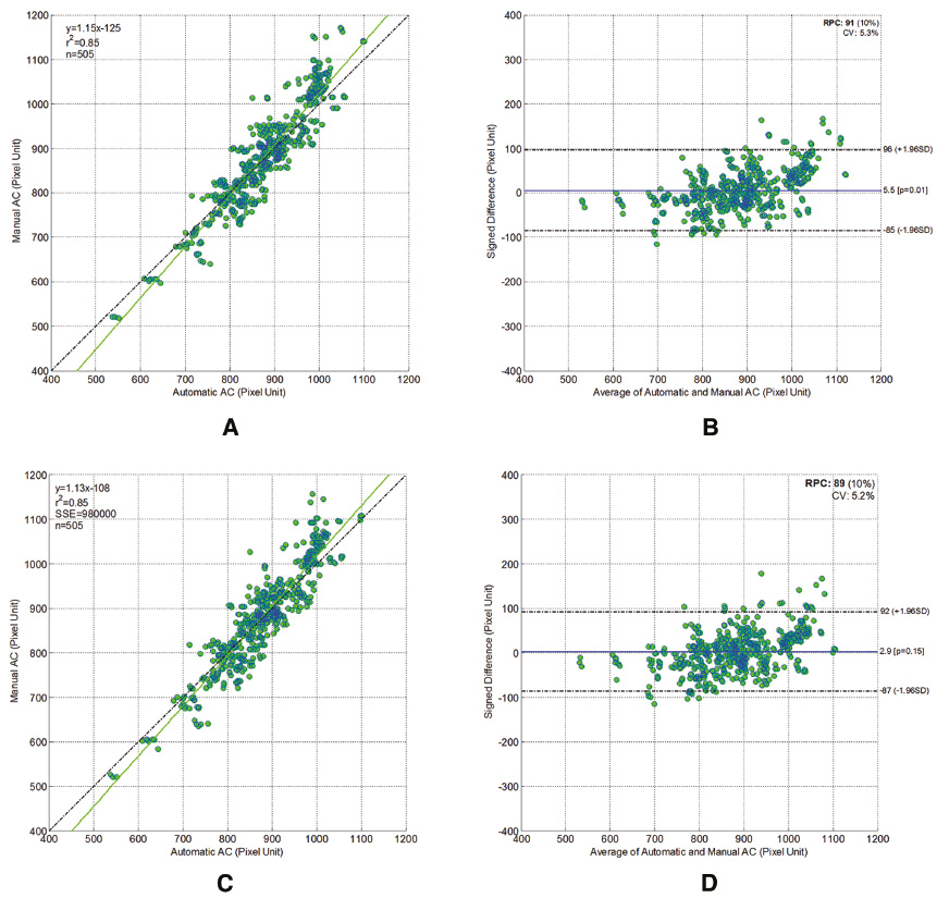
Then, in order to assess the accuracy of our method, the automatic segmentation for HC was plotted against the manually delineated HC in a Bland-Altmann plot [Figure 11(B), (D)]. Similarly, the automatic segmentation for AC was also plotted against the manually delineated HC in a Bland-Altmann plot [Figure 11(B), (D)].
Comparison with learning-based and shape model-based methods
In order to quantitatively evaluate the efficacy of our proposed method, we compared our method with a pixel-wise prediction method (learning-based method) and boundary-driven segmentation method (shape model-based method). Specifically, the distance learning algorithm (Dist-Learn) introduced in [5] stands for the pixel-wise prediction method. For the boundary-driven methods, the state-of-the-art segmentation algorithm (DoGEll) proposed by [3] was compared in the fetal head segmentation. For fair comparison, the inputs of all the evaluated methods are automatically localized ROI images. To present comprehensive segmentation evaluation, four region-based metrics (precision, conform, recall and dice) and three distance-based metrics (MSD, ASD and RMSD) are adopted in our evaluation, referring to delineations of the two experienced doctors.
For Dist-Learn and our proposed method, performances in the final levels are considered. Detailed results are reported in Table 1 and Table 2, and we can see that, our proposed method achieves the best performances in almost all the metrics in both the fetal head and abdomen segmentation tasks (except the region-based metric “recall”). Because of the more significant appearance changes in both the outer and inner parts of the fetal head than that in the abdomen (Figure 1), the Dist-Learn method suffers more from the ambiguous labeling in fetal head US images, and performs worse on fetal head segmentation than fetal abdomen segmentation.
Table 1 Quantitative Evaluation of Fetal Head Ultrasound Image Segmentation
| Method | Region-Based | Distance-Based | |||||
|---|---|---|---|---|---|---|---|
| Dice | Conform | Precision | Recall | MSD | RMSD | ASD | |
| Dist-Learn | 87.0 ± 5.6 | 69.1 ± 15.5 | 83.1 ± 7.3 | 91.6 ± 5.6 | 13.0 ± 5.2 | 6.2 ± 2.4 | 5.1 ± 2.0 |
| DoGELL | 94.2 ± 5.2 | 86.9 ± 14.3 | 98.7 ± 5.4 | 90.6 ± 7.2 | 5.3 ± 5.0 | 2.6 ± 2.5 | 2.1 ± 1.8 |
| Our proposed | 95.5 ± 2.9 | 90.3 ± 7.1 | 97.0 ± 3.1 | 94.1 ± 4.8 | 4.8 ± 2.9 | 2.2 ± 1.4 | 1.7 ± 1.1 |
ASD: average surface distance; MSD: maximum surface distance; RMSD: root mean square surface distance. The bold values denote the best result in each metric.
Table 2 Quantitative Evaluation of Fetal Abdomen Ultrasound Image Segmentation
| Method | Region-Based | Distance-Based | |||||
|---|---|---|---|---|---|---|---|
| Dice | Conform | Precision | Recall | MSD | RMSD | ASD | |
| Dist-Learn | 90.9 ± 3.3 | 79.7 ± 8.3 | 88.3 ± 5.6 | 94.1 ± 5.2 | 10.5 ± 3.7 | 4.9 ± 1.7 | 4.0 ± 1.5 |
| Our proposed | 91.9 ± 3.3 | 82.0 ± 8.4 | 92.3 ± 5.1 | 91.9 ± 5.5 | 8.8 ± 3.5 | 4.3 ± 1.8 | 3.6 ± 1.5 |
ASD: average surface distance; MSD: maximum surface distance; RMSD: root mean square surface distance. The bold values denote the best result in each metric.
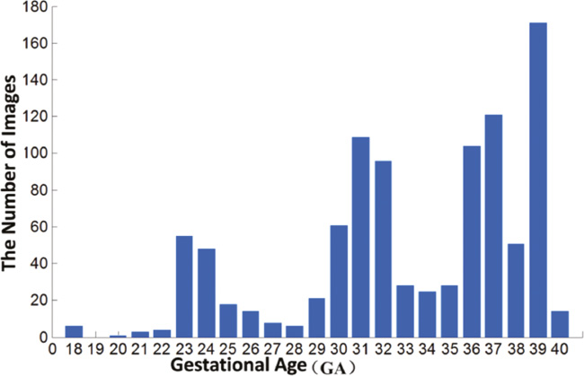
Compared to our proposed method, the specific designed ellipse model in the DoGEll method becomes less competitive in fetal head segmentation. It is probably due to the fact that the testing dataset is complex and broad, as shown in Figure 13.
Figure 13 GA distribution of the fetal ultrasound testing dataset.
Conclusion
In this paper, we propose a general framework for automatic, accurate segmentation of fetal anatomical structures in 2D US images. Our proposed method benefits a lot from the patch-wise joint classification presented by SRFs and the successive detail enhancement from different visual levels provided by the SACM. Our proposed framework was validated on two challenging tasks: fetal head and abdomen segmentation, and achieved the most accurate results in both.
Acknowledgment
This work was assisted by the National Natural Science Funds of China (Nos. 61571304, 61701312, 81571758 and 81771922) and the National Key Research and Develop Program (No. 2016YFC0104703).
References
- Sarris I, Ioannou C, Chamberlain P, Ohuma E, Roseman F, et al. Intra- and interobserver variability in fetal ultrasound measurements. Ultrasound Obstet Gynecol 2012;39:266-73. [PMID: 22535628 DOI: 10.1002/uog.10082]
- Alison Noble J. Reflections on ultrasound image analysis. Med Image Anal 2016;33:33-7. [PMID: 27503078 DOI: 10.1016/j.media.2016.06.015]
- Yu J, Wang Y, Chen P, Shen Y. Fetal abdominal contour extraction and measurement in ultrasound images. Ultrasound Med Biol 2008;34:169-82. [PMID: 17935873 DOI: 10.1016/j.ultrasmedbio.2007.06.026]
- Yu J, Wang Y, Chen P. Fetal ultrasound image segmentation system and its use in fetal weight estimation. Med Biol Eng Comput 2008;46:1227-37. [PMID: 18850125 DOI: 10.1007/s11517-008-0407-y]
- Ciurte A, Bresson X, Cuisenaire O, Houhou N, Nedevschi S, et al. Semi-supervised segmentation of ultrasound images based on patch representation and continuous min cut. PLoS One 2014;9:e100972. [PMID: 25010530 DOI: 10.1371/journal.pone.0100972]
- Jardim SVB, Figueiredo MAT. Automatic contour estimation in fetal ultrasound image. In Proc IEEE Int Conf Image Process 2003;3:II-1065-8. [DOI: 10.1109/ICIP.2003.1246869]
- Wang W, Qin J, Zhu L, Ni D, Chui YP, et al. Detection and measurement of fetal abdominal contour in ultrasound images via local phase information and iterative randomized hough transform. Biomed Mater Eng 2014;24:1261-7. [PMID: 24212021 DOI: 10.3233/BME-130928]
- Wang CW. Automatic entropy-based femur segmentation and fast length measurement for fetal ultrasound images. In Proc. IEEE Advanced Robotics and Intelligent Systems (ARIS). 2014. pp. 1-5. DOI: 10.1109/ARIS.2014.6871490]
- Foi A, Maggioni M, Pepe A, Rueda S, Noble JA, et al. Difference of Gaussians revolved along elliptical paths for ultrasound fetal head segmentation. Comput Med Imaging Graph 2014;38:774-84. [PMID: 25450760 DOI: 10.1016/j.compmedimag.2014.09.006]
- Gall J, Lempitsky V. Class-specific hough forests for object detection. In: Decision forests for computer vision and medical image analysis. Springer London; 2013. pp. 143-57. DOI: 10.1007/978-1-4471-4929-3_11]
- Namburete AIL, Stebbing RV, Kemp B, Yaqub M, Papageorghiou AT, et al. Learning-based prediction of gestational age from ultrasound images of the fetal brain. Med Image Anal 2015;21:72-86. [PMID: 25624045 DOI: 10.1016/j.media.2014.12.006]
- Gao Y, Shen D. Context-aware anatomical landmark detection: application to deformable model initialization in prostate CT images. In International Workshop on Machine Learning in Medical Imaging. Springer International Publishing; 2014. pp. 165-73. DOI: 10.1007/978-3-319-10581-9_21]
- Gao Y, Wang L, Shao Y, Shen D. Learning distance transform for boundary detection and deformable segmentation in CT prostate images. In International Workshop on Machine Learning in Medical Imaging. Springer International Publishing; 2014. pp. 93-100. DOI: 10.1007/978-3-319-10581-9_12]
- Yaqub M, Javaid MK, Cooper C, Noble JA. Investigation of the role of feature selection and weighted voting in random forests for 3-D volumetric segmentation. IEEE Trans Med Imaging 2014;33:258-71. [PMID: 24108712 DOI: 10.1109/TMI.2013.2284025]
- Kontschieder P, Bulo SR, Bischof H, Pelillo M. Structured class-labels in random forests for semantic image labelling. In Proceedings of the IEEE International Conference on Computer Vision. IEEE; 2011. pp. 2190-7. DOI: 10.1109/ICCV.2011.6126496]
- Dollár P, Zitnick CL. Structured forests for fast edge detection. In Proceedings of the IEEE International Conference on Computer Vision. 2013. pp. 1841-8. DOI: 10.1109/ICCV.2013.231]
- Domingos JS, Stebbing RV, Leeson P, Alison Noble J. Structured random forests for myocardium delineation in 3D echocardiography. In International Workshop on Machine Learning in Medical Imaging. Springer International Publishing. 2014. pp. 215-22. DOI: 10.1007/978-3-319-10581-9_27]
- Carneiro G, Georgescu B, Good S, Comaniciu D. Detection and measurement of fetal anatomies from ultrasound images using a constrained probabilistic boosting tree. IEEE Trans Med Imaging 2008;27:1342-55. [PMID: 18753047 DOI: 10.1109/TMI.2008.928917]
- Ni D, Yang Y, Li S, Qin J, Ouyang S, et al. Learning based automatic head detection and measurement from fetal ultrasound images via prior knowledge and imaging parameters. In IEEE 10th International Symposium on Biomedical Imaging. 2013. pp. 772-5. DOI: 10.1109/ISBI.2013.6556589]
- Zhang L, Chen S, Chin CT, Wang T, Li S. Intelligent scanning: automated standard plane selection and biometric measurement of early gestational sac in routine ultrasound examination. Med Phys 2012;39:5015-27. [PMID: 22894427 DOI: 10.1118/1.4736415]
- Ni D, Yang X, Chen X, Chin C-T, Chen S, et al. Standard plane localization in ultrasound by radial component model and selective search. Ultrasound Med Biol 2014;40:2728-42. [PMID: 25220278 DOI: 10.1016/j.ultrasmedbio.2014.06.006]
- Riha K, Masek J, Burget R, Benes R, Zavodna E. Novel method for localization of common carotid artery transverse section in ultrasound images using modified viola-jones detector. Ultrasound Med Biol 2013;39:1887-902. [PMID: 23849387 DOI: 10.1016/j.ultrasmedbio.2013.04.013]
- Tu Z, Bai X. Auto-context and its application to high-level vision tasks and 3D brain image segmentation. IEEE Trans Pattern Anal Mach Intell 2010;32:1744-57. DOI: 10.1109/TPAMI.2009.186]
- Criminisi A, Shotton J. Decision forests for computer vision and medical image analysis. New York: Springer; 2013. p. 387. DOI: 10.1007/978-1-4471-4929-3]
- Rueda S, Fathima S, Knight CL, Yaqub M, Papageorghiou AT, et al. Evaluation and comparison of current fetal ultrasound image segmentation methods for biometric measurements: a grand challenge. IEEE Trans Med Imaging 2014;33:797-813. [PMID: 23934664 DOI: 10.1109/TMI.2013.2276943]
- Nho JH, Lee YK, Kim HJ, Ha YC, Suh YS, et al. Reliability and validity of measuring version of the acetabular component. J Bone Joint Surg 2012;94:32-6. [PMID: 22219244 DOI: 10.1302/0301-620X.94B1.27621]